Getting Started with Scilab

Introducing one of the larger scientific lab packages for Linux.
Scilab is meant to be an overall package for numerical science, along the lines of Maple, Matlab or Mathematica. Although a lot of built-in functionality exists for all sorts of scientific computations, Scilab also includes its own programming language, which allows you to use that functionality to its utmost. If you prefer, you instead can use this language to extend Scilab's functionality into completely new areas of research. Some of the functionality includes 2D and 3D visualization and optimization tools, as well as statistical functions. Also included in Scilab is Xcos, an editor for designing dynamical systems models.
Several options exist for installing Scilab on your system. Most package management systems should have one or more packages available for Scilab, which also will install several support packages. Or, you simply can download and install a tarball that contains everything you need to be able to run Scilab on your system.
Once
it's installed, start the GUI version of Scilab with
the scilab command. If you installed Scilab via tarball, this command will
be located in the bin subdirectory where you unpacked the tarball.
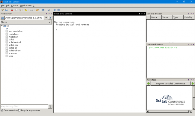
When it first starts, you should see a full workspace created for your project.

Figure 1. When you first start Scilab, you'll see an empty workspace ready for you to start a new project.
On the left-hand side is a file browser where you can see data files and Scilab scripts. The right-hand side has several panes. The top pane is a variable browser, where you can see what currently exists within the workspace. The middle pane contains a list of commands within that workspace, and the bottom pane has a news feed of Scilab-related news. The center of the workspace is the actual Scilab console where you can interact with the execution engine.
Let's start with some basic mathematics—for example, division:
--> 23/7
 ans  =

   3.2857143
As you can see, the command prompt is -->, where you enter the
next command to the execution engine. In the variable browser, you
can see a new variable named ans that contains the results of the
calculation.
Along with basic arithmetic, there is also a number of built-in functions. One thing to be aware of is that these function names are
case-sensitive. For example, the statement sqrt(9) gives the answer
of 3, whereas the statement SQRT(9) returns an error.
There also are built-in constants for numbers like e or pi. You can use them in statements, like this command to find the sine of pi/2:
--> sin(%pi / 2)
 ans  =

   1.
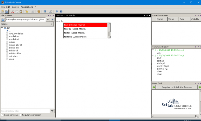
If you don't remember exactly what a function name is, but you remember how it starts, you can use the tab-completion functionality in the Scilab console. For example, you can see what functions start with "fa" by typing those two letters and then pressing the tab key.

Figure 2. Use tab-completion to avoid typos while typing commands in the Scilab console.
You can assign variables with the "=" symbol. For example,
assign your age to the age variable with:
--> age = 47
 age  =

   47.
You then can access this variable directly:
--> age
 age  =

   47.
The variable also will be visible in the variable browser pane. Accessing
variables this way basically executes the variable, which is also why you
can
get extra output. If you want to see only the value, use
the disp() function, which provides output like the following:
--> disp(age)

   47.
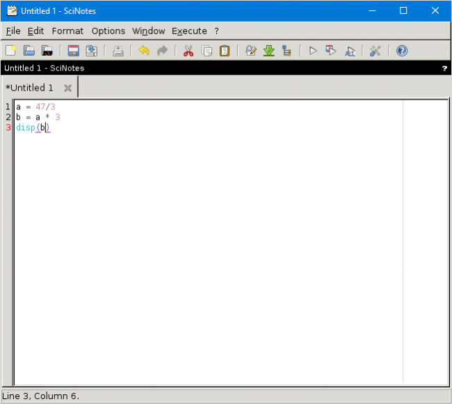
Before moving onto more complex ideas, you'll need to move out of the console. The advantage of the console is that statements are executed immediately. But, that's also its disadvantage. To write larger pieces of code, you'll want to use the included editor. Click the Applications→SciNotes menu item to open a new window where you can enter larger programs.

Figure 3. The SciNotes application lets you write larger programs and then run them within Scilab as a single unit.
Once you've finished writing your code, you can run it either by clicking the run icon on the toolbar or selecting one of the options under the Execute menu item. When you do this, SciNotes will ask you to save your code to a file, with the file ending ".sce", before running. Then, it gets the console to run this file with the following command:
exec('/home/jbernard/temp/scilab-6.0.1/bin/test1.sce', -1)
If you create or receive a Scilab file outside of Scilab, you can run it yourself using a similar command.
To build more complex calculations, you also need a way to make comparisons and loop over several calculations. Comparisons can be done with either:
if .... then
   stmts
end
or:
if .... then
   stmts
else
   stmts
end
or:
if .... then
   stmts
elseif .... then
   stmts
else
   stmts
end
As you can see, the if and elseif lines need to
end with then. You can
have as many elseif sections as you need for your particular case. Also,
note that the entire comparison block needs to end with the
end statement.
There
also are two types of looping commands: for loops and
while loops. As
an example, you could use the following to find the square roots
of the first 100 numbers:
for i=1:100
    a = sqrt(i) disp(a)
end
The for loop takes a sequence of numbers, defined by
start:end,
and each value is iteratively assigned to the dummy variable i. Then
you have your code block within the for loop and close it with the
statement end.
The while loop is similar, except it uses a comparison
statement to decide when to exit the loop.
The last quick item I want to cover is the graphing functionality available within Scilab. You can create both 2D and 3D graphs, and you can plot data files or the results of functions. For example, the following plots the sine function from 0 to pi*4:
t = linspace(0, 4 * %pi, 100) plot(t, sin(t))
Figure 4. Calling the plot function opens a new viewing window where you can see the generated graphs.
You can use the linspace command to generate the list of values over
which the function will be executed. The plot function opens a new
window to display the resultant graph. Use the commands under
the Edit menu item to change the plot's details before saving the
results to an image file.
You can do 3D graphs just as simply. The following plots a parametric curve over 0 to 4*pi:
t=linspace(0,4*%pi,100); param3d(cos(t),sin(t),t)
Figure 5. Generating 3D graphs is as easy as generating 2D plots, as this parametric curve example shows.
This also opens a new plotting window to display the results. If the default view isn't appropriate, click Tools→2D/3D Rotation, and with this selected, right-click on the graph and rotate it around for a better view of the result.
Scilab is a very powerful tool for many types of computational science. Since it's available on Linux, macOS and Windows, it's a great option if you're collaborating with other people across multiple operating systems. It might also prove to be a effective tool to use in teaching environments, giving students access to a powerful computational platform for no cost, no matter what type of computer they are using. I hope this short article has provided some ideas of how it might be useful to you. I've barely covered the many capabilities available with Scilab, so be sure to visit the main website for a number of good tutorials.


