Nightfall on Linux
I've looked at general astronomy programs in the past that are helpful for many tasks you might need to do in your stargazing career. But, several specific jobs are more complicated and require specialized software to make relevant calculations, so here, let's take a look at Nightfall.
Nightfall is a program that can handle calculations involving binary star systems. It can animate binary star systems, taking into account not only orbital speeds but also rotational motion and the changing shape of stars due to their close positions. You can model what it would look like and what kind of light curves you would register when observing a binary system. You even can take a set of actual observational data and find a best-fit model for the system you are studying.
Most distributions don't include a package for Nightfall, so you need to build it from source. There are several dependencies, so the instructions following assume that you are using a Debian-based distribution. If you are using something else, you should be able to find the comparable packages for your distribution of choice. To install the dependencies, run the command:
sudo apt-get install libgtk2.0-0 libgtk2.0-dev gnuplot
Nightfall also includes the ability to use OpenGL to handle 3D rendering of animations of the binary systems you want to model. If you want to use OpenGL, you also need to install:
sudo apt-get install libgl1-mesa-dev freeglut3-dev
 ↪libgtkgl2.0-dev libjpeg62-dev
Once all of the requirements are installed, you can install Nightfall itself. You should change directory into a temporary or source directory where you can do the unpacking and build the code. Once you are there, download the latest version of Nightfall with:
wget https://www.la-samhna.de/nightfall/nightfall-1.88.tar.gz
Then, unpack it with:
tar xvzf nightfall-1.88.tar.gz
When you go to configure Nightfall, you probably will want to include
the openmp option. This allows Nightfall to use the multiple CPUs
you probably have in your machine to speed up the calculations
involved. You can build and install Nightfall with:
./configure --enable-openmp make sudo make install
This installs Nightfall under the /usr/local directory. You then can start Nightfall with:
nightfall -U
The -U option is necessary to force the GUI to be used interactively.
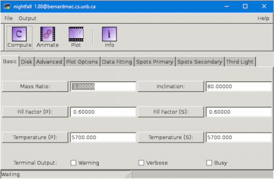
Figure 1. The GUI lets you configure all kinds of options within Nightfall to set up your model.
Now that Nightfall is up and running, you will start to see just how much control you have over the model that is being simulated. The first tab is where you can set up the core parameters for your binary system model. You can set the mass ratio and the inclination of the two stars. You also can set the surface temperatures and the Roche lobe filling factors for each of the stars. The temperature helps define their luminosities, and the Roche lobe filling factors define the distortion of the stars.
Depending on the exact conditions, you may have an accretion disk of material around the central star. The second tab lets you set the type of accretion disk (that is, how it interacts with the central star), along with more physical parameters like the inner and outer diameters and the temperature.
The advanced tab allows you to set some less obvious parameters for your model, such as the eccentricity for the orbiting star and whether you also need to model the atmosphere.
Now you can click on the Compute button at the top of the window, and on most modern machines, it goes pretty quickly. Once the calculations are done, you can plot the output from the system you just modeled.
The Output menu item on the menu bar at the top gives you several options on how to display the calculated results. The first entry is PlotCurve, which draws the light curve as seen from a distant observer. Gnuplot is used to draw the actual plot of the visible amount of light that is seen.
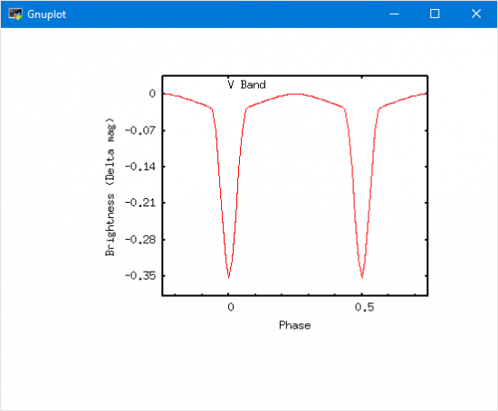
Figure 2. Once the calculation is done, you can plot the observed light curve.
The second output option is to select ViewGeometry. This plot shows you how the stars themselves are distorted within their orbits.
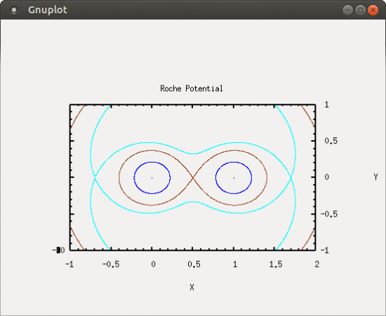
Figure 3. You can plot the geometry of the stars within the binary system.
The StarView menu item presents a view of how the binary system would look from your observation point. A control box also pops up that allows you to change the inclination of the orbital plane and the phase of the orbit.
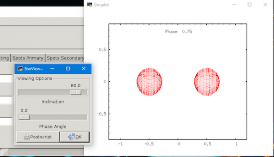
Figure 4. Selecting StarView lets you see the binary system from some distance away.
The RocheSlicer menu item provides a way to visualize just how distorted the stars become. A control box also pops up that lets you select various slices through the star system.
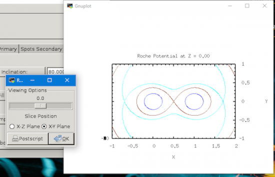
Figure 5. The RocheSlicer lets you investigate the distortions in the stars of your binary system.
The last menu item is the DataSheet option. This option pops up a new window with a text description of the results of all of the calculations that were made.
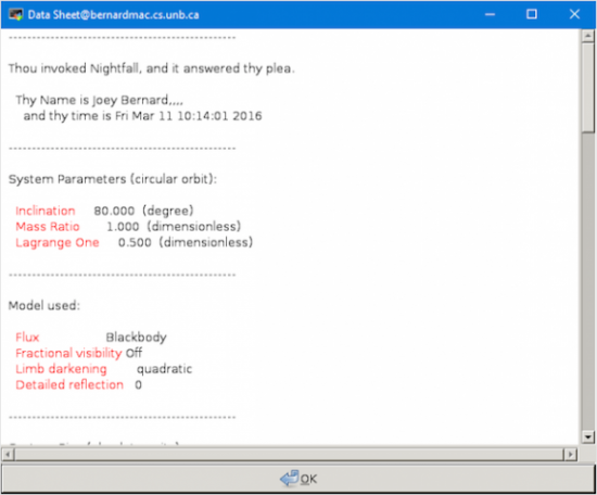
Figure 6. The DataSheet gives you the detailed numerical results of your simulation.
One of the keys in science is being able to reproduce your results, both experimental and computational. With this in mind, you can save the model you just ran and load it again later. These models are saved as configurations by clicking the menu item File→Save Configuration. You can load previous models by clicking the menu item File→Open config file. If you compiled and installed Nightfall using the instructions above, you will have a number of example configurations available that you can play with as well.
Nightfall is not only useful in determining what a given binary star system would look like, but you also can feed in your own observational data and calculate a best-fit model to those observations. You can load your observational data by clicking the menu item File→Open data file. Again, if you compiled and installed Nightfall following the instructions above, you will have several sample data files that you can load. You probably should click on the menu item File→Clear memory first. Once the data is loaded, select the Data Fitting tab in the main window. You then need to select the Mass and/or Separation buttons as parameters for the fitting. Then, select the FIT with tolerance button, using the tolerance you enter within the text box. You also can choose whether to use simulated annealing or Monte Carlo methods. You may want to do some research to see how active astronomers use these parameters to find best-fit models.
The last thing to notice is that almost everything you can do with the GUI is also doable with command-line options. This means you can generate many different models with different sets of parameters and generate the relevant plots and output data automatically. This way, you can farm out the work to some cluster of machines (but that's moving into the realm of "professional" astronomy and beyond the scope of this article).


