GIS on Linux with SAGA
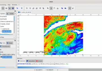
In this article, I want to look at a GIS option available for Linux—specifically, a program called SAGA (System for Automated Geoscientific Analyses). SAGA was developed at the Department of Physical Geography in Germany. It is built with a plugin module architecture, where various functions are provided by individual modules. A very complete API is available to allow users to extend SAGA's functionality with newly written modules. I take a very cursory look at SAGA here and describe a few things you might want to do with it.
Installing SAGA should be as easy as looking at the software repository for your favourite distribution. For Debian-based distros, you can install it with the command:
sudo apt-get install saga
When you first start it, you get a blank workspace where you can begin your project.
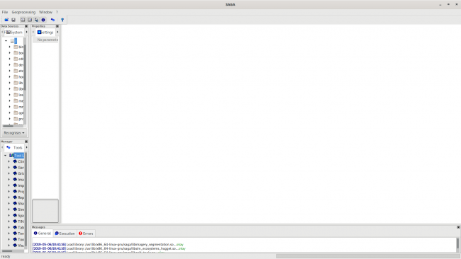
Figure 1. SAGA starts up with a central project window, several tool panes on the left and console messages at the bottom.
Two major categories of data sets are available that you can use within your projects: satellite imagery and terrain data. The tutorial website provides detailed walk-throughs that show how you can get access to these types of data sets for use in your own projects. The tutorial website also has sections on some of the processing tools available for doing more detailed analysis.
SAGA understands several data file formats. The typical ones used in GIS, like SHP files or point clouds, are the default options in the file selector window. You can work with these types of data, or satellite imagery or terrain data.
Let's start by looking at terrain analysis in SAGA. You'll need digital elevation data, in DEM format, which is available from the SRTM Tile Grabber site. You will get a zip file for each region you select, and these zip files contain geotiff files for the selected regions.
Load the geotiff file by clicking File→Open. By default, it will show only the common project file formats. To locate your downloaded geotiff files, you'll need to change the filter at the bottom of the file selector window to be all files. Once it is loaded, it will show up in the list of data sources in the bottom-left window pane.
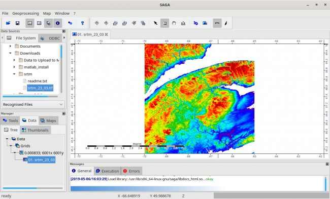
Figure 2. You can load data sources, such as geotiffs, into your project.
You may find that the default layout is a bit crowded, so you may want to close some of the detail panes, as I did in the screenshot here. By default, the file is simply added to the list of data sources in the data manager pane in the bottom left of the window, and nothing is displayed. To view the newly added data, you can right-click on the entry in the data manager and select "Add to Map". Several other options are available when you right-click the data source. For example, you can click on "Spatial Reference" to get details about the projection and so on.
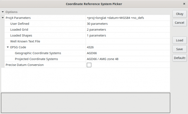
Figure 3. You can play with projection settings for a data source.
Moving to the "Map" tab of the bottom-right pane, you can see the current list of maps and their layers. Right-clicking on the layers provides only viewing options, like what layers lie above or below other layers. Right-clicking on the map provides a bit more functionality. You can save maps as images or even copy them to the clipboard to be used in some other application. You change the overall view to either a 3D view or a print layout. You even can add extra items to your map, such as a base map or a graticule. You also can adjust the order of the layers, in order to have all of the appropriate information displayed correctly. Several other tools are available under the "map" menu item at the top of the window.
When you click the "Geoprocessing" menu item, you'll see the massive list of tools available to do processing tasks on the data that you have imported. Some of them are basic, while others are very computationally intensive. For example, if you click Terrain Analysis→Basic Terrain Analysis, it can sit and run for quite a while. You will select single analysis tools if you want to look at some specific items. For example, you could look at the solar radiation by clicking Geoprocessing→Terrain Analysis→Lighting→Potential Incoming Solar Radiation.
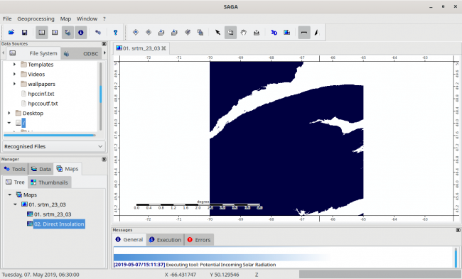
Figure 4. You can run tools that provide additional layers to be displayed in your map.
As you can see, a very dense tree of tools is available. Many of these tools also are available under the "Tools" tab in the bottom-left pane. You simply find the tool in question and double-click it. You may, however, discover that it's difficult to find a specific tool. If that's the case, click Geoprocessing→Find and Run Tool, and you'll get a pop-up window where you can look for something specific.
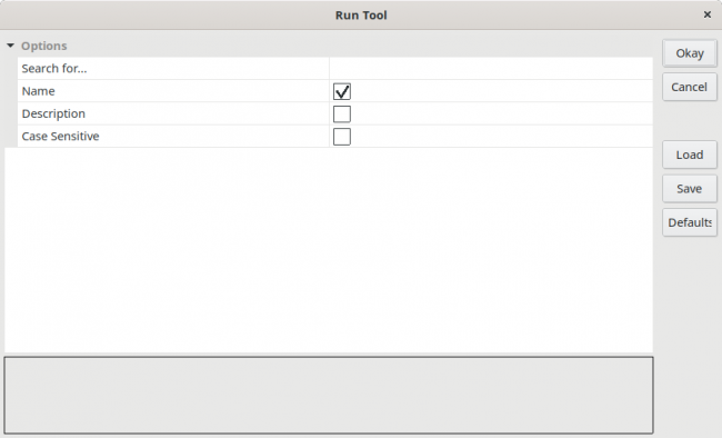
Figure 5. You can do a search for a specific tool, rather than navigating through the menus.
To get a better idea of what you can do, the SAGA tutorial site includes a set of complete application examples that walk you through entire workflows. For instance, the first one in the list is assessing sediment flows from a point field survey. It explains how to import data from a CSV file, apply coordinate transformations and visualize the resulting data. It then walks through how to apply a hydrological analysis tool to better understand how the sediment flow happens based on the terrain information.
I hope this short article whets your appetite for using GIS in your own projects. I've covered only a small taste of everything you can do with SAGA, and as with many open-source projects, you always can add extra functionality as needed, which will be loaded as shared libraries that provide additional tools.


