Getting Good Vibrations with Linux

Vibrations and wave motions describe many different physical systems. In fact, most systems that dissipate energy do so through waves of one form or another. In this article, I take a look at gvb (Good ViBrations, https://www.pietrobattiston.it/gvb), a Linux application you can use to visualize and model wave motion and vibrations.
Installation should be relatively easy. It already should exist in the packaging system of most distributions. For example, on Debian-based systems, you can install it with this:
sudo apt-get install gvb
You will notice that a large number of Python requirements also are installed. This gives you an idea of what you need as requirements if you want to build gvb from source.
Now that you have gvb and its requirements installed, you can start
it by running the command gvb. When it starts, you will
see a main display window with a pane on the right-hand side with
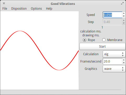
calculation options. In the main window, there will be a starting sine
wave form.

Figure 1. When you first start gvb, you will see a sine wave ready to start modeling.
Just to make sure that everything is working, you can click on the start button in the right-hand pane. This starts the calculations used to model the wave motion and shows each time step in the main display window. You should see the evolution of a basic sine wave happening.
Let's use this starting waveform to play with some of the available calculation options. The first option is the speed of the wave. You can change this while the wave is being modeled and animated, so you can see in real time how the wave changes with a different speed.
Below the start button are three available options. The calculation drop-down lets you change the algorithm used to do the calculations. The default is eig, and the other three methods are quad, naif and naif matrix. When you select any of the other three methods, the step size option at the top of the pane becomes active.
You then can change the size of the steps used in calculating the wave motion. You can set the number of frames per second to display. The higher this value is, the smoother your wave animation will be. You probably won't notice any improvement beyond 30 frames per second, simply due to the limits of human vision.
The last option allows you to change what graphics are actually rendered in the display. Wave shows the waveform itself. Temp displays a color map representing the amplitude with different colors. Speed displays the waveform, like Wave, but it also includes a series of bars along the wave indicating the magnitude of the speed at those points along the wave. This display helps students get a feeling for how fast the different parts of the wave are moving.
Before going on, it would be worth spending a few minutes to take a cursory
look at the types of calculations gvb can do. The default calculation
method is eig. This method actually uses the eig() function found
in the linalg part of NumPy. This uses the plane wave expansion method
to get an eigenvalue formulation of the problem and solve that.
The naif calculation method is a naive method. It simply takes the current amplitude of the wave at some point and calculates how far it should travel based on a linear application of the current speed at that point.
The naif matrix method just tries to speed up the naif method by treating the wave as a vector rather than point by point. Neither of these two methods should be used for any reason other than to see just how bad they are.
The last method is quad. This method expands on the simplistic speed calculation of the naif method with a more accurate method. In most cases, you simply will want to use the eig method, as it is the most accurate for most situations.
Up until now, I've only been discussing a sinusoidal wave on a string. But really interesting things happen when you can look at other starting waveforms. There are a series of pre-programmed waveforms available for you under the menu entry Disposition→1 dimension: precooked. Here you will find more than a dozen available options.
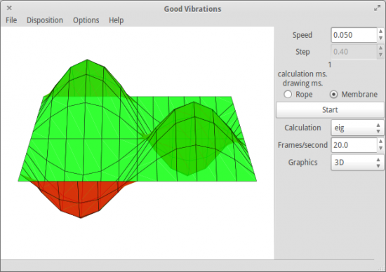
You also may have noticed that there is also an entry for two-dimensional precooked options. That's right, gvb can model waves on a membrane as well.

Figure 2. You even can model waves on a membrane with gvb.
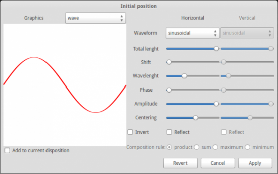
If you select one of these precooked options, you should notice that the graphics option is changed to 3-D, and the type of drawing is changed from rope to membrane. Clicking the start button will show you how the starting waveform propagates across the given membrane. Under the Disposition menu entry, there also are entries for advanced one- and two-dimensional systems. Selecting one of these will pop up a new window where you can set the various parameters for your own model.

Figure 3. The advanced window allows you to create your own customized waveforms.
You still are limited to sinusoidal, triangular, square and peak waves as your base forms. If you have something even more complicated in mind, you actually can define the amplitude and speed at each point in a text file. For example, to model a string, the text file will have three lines. The first line will contain the shape—in this case, the number of points along the string. The second line will contain a series of amplitude values, comma-separated, one for each point. The third line will contain a series of speed values, comma-separated, one for each point. You next need to end the file with a new-line character at the end. Then, you can read this into gvb to provide your starting waveform. This gives you maximum flexibility. You can do the equivalent two-dimensional input file if you want to model a membrane rather than a string.
One final thing you may want to do with gvb is generate a movie of the wave you are modeling. Selecting the menu entry Options→Save frames as png will pull up a file selection window. You need to choose a directory to store all of the image files for each frame of the animation. Once this is done and you click the start button, a PNG file will be written out for each frame. In order to generate a movie out of those, you need to have FFmpeg installed on your system. Then, all you have to do is change directory to the spot where gvb is writing out these image files and run the command:
ffmpeg -i *.png video.mp4
Now you have a video file that you can share displaying the wave evolution that you are modeling.
As you have seen, gvb can be a very fun application to use. It especially gives students a more intuitive feel for how waves behave, in both one and two dimensions. The ability to visualize the speeds for various sections also helps conceptualize the physics involved. Hopefully, the teachers out there will keep gvb in mind when they are planning their next science class to help students understand wave mechanics.


